HARFA: SCREENSHOTS AND TUTORIALS: SLOPE ANALYSIS   Fractal Analysis Slope Analysis Real fractals can be infinitely zoomed in or out and none of their characteristic properties will change. They are scale independent. But objects that can be studied using HarFA are not pure fractals, they are images of fractals. Images of fractals are scale independent just in some interspace of zooming. When the image of fractal is enlarged, (when size of overlaid mesh is too small), no fractal but a mosaic composed from white and black elements (pixels) can be seen. When the fractal is reduced too much, (when square size is inadequately large), the fractal will disappear in white background. The distortion can be seen in fractal functions (NB(r) = DB(log(1/r)) + kB, NBW(r) = DBW(log(1/r)) + kBW, NW(r) = DW(log(1/r)) + kW) as a disturbance of linearity. The exact determination of a fractal dimension requires the linear part of the function (fig. 1).          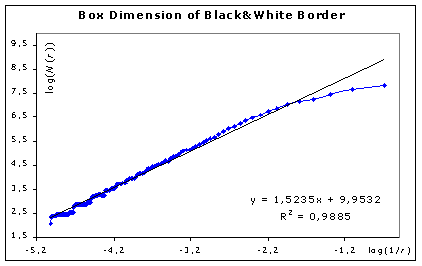Fig. 1: Typical structure of function NBW(r) = DBW(log(1/r)), disturbance of linearity due to image of fractal. It is fairly complicated task. There are tools described in literature to accomplish this goal, but they are too difficult and time and computationally expansive. So, in HarFA, there is easier tool, which can help to find linear part of function NBW(r) = DBW(log(1/r) - Slope Analysis. How it works? User must specify Size of Tested Area (20 as starting value is recommended). Data from fig. 1. are sequently loaded into memory and their slope and regression coefficient is computed. It means, that when we have, let's say, 60 data values pairs (X: log(1/r), Y: N(r), where r - square size, N - count of black&white squares), first we load data 1.-20., we establish their slope and regression coefficient, second we load data 2.-21., third 3.-22., 4.-23. and so on. Slopes of these segments are written to chart (see fig. 2) as a function of ln(1/r) of the first value in segment, and colorized according it's correlation coefficient. Linear part will distinguish by constant part on new dependency (there are same, or almost same slopes) and by high correlation (marked by red tint or white color - correlation larger than 0.999).          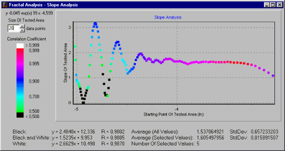Fig. 2: Slope Analysis: Linear Part is in the interspace from -3.34 to -3.73 (x-values), is marked by bright red tint, It corresponds to values of mesh 1/exp-3.34 = 28 to 1/exp-3.73 = 42, it means linear part between values of squares sizes from 28 to (42 + 20). Resulting Box Dimension should be about 1.606 with standard deviation (determined using 25 values (20+5)) 0.016. We can select datapoints by clicking it by mouse and observe standard deviation and average of selected datapoints. Deselecting is performed by clicking Average (Selected Value) label. Previous Next